Logging and Analysis
Monty Loggers
To manage the logging for an experiment you can specify the handlers that should be used in the logging config. The logging config has two fields for handlers. One for monty_handlers and one for wandb_handlers. The latter will start a wandb session if it does not contain an empty list. The former can contain all other non-wandb handlers.
List of all Logging Handlers
| Class Name | Description |
|---|---|
| MontyHandler | Abstract handler class. |
| DetailedJSONHandler | Logs detailed information about every step in a .json file. This is for detailed analysis and visualization. For longer experiments, it is not recommended. |
| BasicCSVStatsHandler | Log a .csv file with one row per episode that contains the results and performance of this episode. |
| BasicWandbTableStatsHandler | Logs a table similar to the .csv table to wandb. |
| BasicWandbChartStatsHandler | Logs episode stats to wandb charts. When running in parallel this is done at the end of a run. Otherwise one can follow the run stats live on wandb. |
| DetailedWandbHandler | Logs animations of raw observations to wandb. |
| DetailedWandbMarkedObsHandler | Same as previous but marks the view-finder observation with a square indicating where the patch is. |
Logging to Wandb
When logging to wandb we recommend to runexport WANDB_DIR=~/tbp/results/monty/wandbso the wandb logs are not stored in the repository folder.
The first time you run experiments that log to wandb you will need to set your WANDB_API key using export WANDB_API_KEY=your_key
Analysis
Analyzing Data From monty_handlers
monty_handlersThe plot_utils.py contains utils for plotting the logged data. The logging_utils.py file contains some useful utils for loading logs and printing some summary statistics on them.
Install
analysisoptional dependencies to useplot_utils.pypip install -e .'[analysis]'
There are many ways of visualizing the logged data. Below are just some commonly use functions as examples but to get a full picture it is best to have a look at the functions in logging_utils.py and plot_utils.py.
Loading Logged Data
The easiest way to load logged data is using the load_stats function. This function is useful if you use the DetailedJSONHandler or the BasicCSVStatsHandler or simply want to load learned models. You can use the function parameters to load only some of the stats selectively. For example, set load_detailed to False if you didn't collect detailed stats in a JSON file or set load_train to False if you only ran validation.
You can Follow Along with this Code
If you ran the
randrot_10distinctobj_surf_agentbenchmark experiment as described in the Running Benchmarks guide, you should be able to run the code below.
import os
from tbp.monty.frameworks.utils.logging_utils import load_stats

pretrain_path = os.path.expanduser("~/tbp/results/monty/pretrained_models/")
pretrained_dict = pretrain_path + "pretrained_ycb_v12/surf_agent_1lm_10distinctobj/pretrained/"

log_path = os.path.expanduser("~/tbp/results/monty/projects/evidence_eval_runs/logs/")
exp_name = "randrot_10distinctobj_surf_agent"
exp_path = log_path + exp_name

train_stats, eval_stats, detailed_stats, lm_models = load_stats(exp_path,
                                                                load_train=False, # doesn't load train csv
                                                                load_eval=True, # loads eval_stats.csv
                                                                load_detailed=False, # doesn't load .json
                                                                load_models=True, # loads .pt models
                                                                pretrained_dict=pretrained_dict,
                                                               )
Alternatively, you can of course always just load the stats files (logged at output_dir specified in the experiment config) using pd.read_csv, json.load, torch.load, or any other library loading function you prefer using.
JSON Logs can get Large Fast
The detailed JSON logs save very detailed information for every step and episode. This includes for example the pixel observations at every step. The .json files can therefore get large very quickly. You should use the
DetailedJSONHandlerwith care and only if needed. Remember to adjust the number of epochs and episodes to be as small as possible.If you need to load a larger JSON file, it makes sense to load it with the
deserialize_json_chunksfunction. This way you can load one episode at a time, process its data, clear memory, and then load the next episode.
Calculating Summary Statistics
We have a couple of useful utils to calculate and print summary statistics from the logged .csv files in logging_utils.py. Below are a few examples of how to use them after loading the data as shown above.
from tbp.monty.frameworks.utils.logging_utils import print_overall_stats

print_overall_stats(eval_stats)
from tbp.monty.frameworks.utils.logging_utils import print_unsupervised_stats

print_unsupervised_stats(train_stats, epoch_len=10)
If you are Following Along you Should see Something like This:
Detected 100.0% correctly overall run time: 104.03 seconds (1.73 minutes), 1.04 seconds per episode, 0.04 seconds per step.
Plotting Object Graphs
When loading the lm_models (either using the load_stats function or torch.load) you get a dictionary of object graphs. Object graphs are represented as torch_geometric.data class instances with properties x, pos, norm, feature_mapping where x stores the features at each point in the graph, pos the locations, norm the surface normal and feature_mapping is a dictionary that encodes which indices in x correspond to which features.
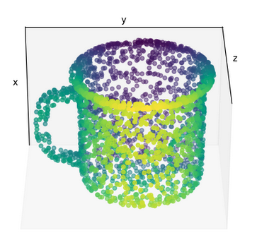
There are a range of graph plotting utils in the plot_utils.py file. Additionally, you can find some more examples of how to plot graphs and how to use the functions in GraphVisualizations.ipynb, EvidenceLM.ipynb, and MultiLMViz.ipynb in the monty_lab repository. Below is just one illustrative example of how you can quickly plot an object graph after loading it as shown above.
import matplotlib.pyplot as plt
from tbp.monty.frameworks.utils.plot_utils_dev import plot_graph

# Visualize the object called 'mug' from the pretrained graphs loaded above from pretrained_dict
plot_graph(lm_models['pretrained'][0]['mug']['patch'], rotation=120)
plt.show()
from tbp.monty.frameworks.utils.plot_utils_dev import plot_graph

# Visualize how the graph for the first object learned (new_object0) looks in epoch 3 in LM_0
plot_graph(lm_models['3']['LM_0']['new_object0']['patch'])
plt.show()
Plotting in 3D
Most plots shown here use the 3D projection feature of matplotlib. The plots can be viewed interactively by dragging the mouse over them to zoom and rotate. When you want to save figures with 3D plots programmatically, it can be useful to set the
rotationparameter in theplot_graphfunction such that the POV provides a good view of the 3D structure of the object.
Plotting Matching Animations
Since Monty is a sensorimotor framework, everything happens as a timeseries of sensing and acting. Therefor, many aspects of the experiment are better visualized as an animation that can show how hypotheses evolve over time. We have a couple of functions to create animations in the plot_utils.py file. Below is one example how this could be applied to data loaded with the code above.
To Follow Along Here You Need to Use the Detailed Logger
Detailed JSON stats are not logged by default since they can get large quickly. To be able to run the following analysis, you need to ensure the experiment
config.logging.monty_handlersconfiguration includesDetailedJSONHandler:config: logging: monty_handlers: - ... - ${monty.class:tbp.monty.frameworks.loggers.monty_handlers.DetailedJSONHandler} - ...It is also recommended to not log too many episodes with the detailed logger so to keep the file size small, we recommend to also update the number of objects tested and number of epochs like this:
# Changes to make to the randrot_10distinctobj_surf_agent config to follow along:
config:
  n_eval_epochs: 1 # <--- Setting n_eval_epochs to 1
  logging:
    monty_handlers:
      - ${monty.class:tbp.monty.frameworks.loggers.monty_handlers.BasicCSVStatsHandler}
      # <--- Include detailed logging handler
      - ${monty.class:tbp.monty.frameworks.loggers.monty_handlers.DetailedJSONHandler}
  eval_env_interface_args:
    object_names:
      - mug # <--- Only testing one object
TODO: Add code for some of the animate functions
Most of them are for the old LMs so probably won't make sense to show them here. Maybe we should even remove them from the code.
There are some animation functions for policy visualizations. @Niels do you think it makes sense to demo them here?
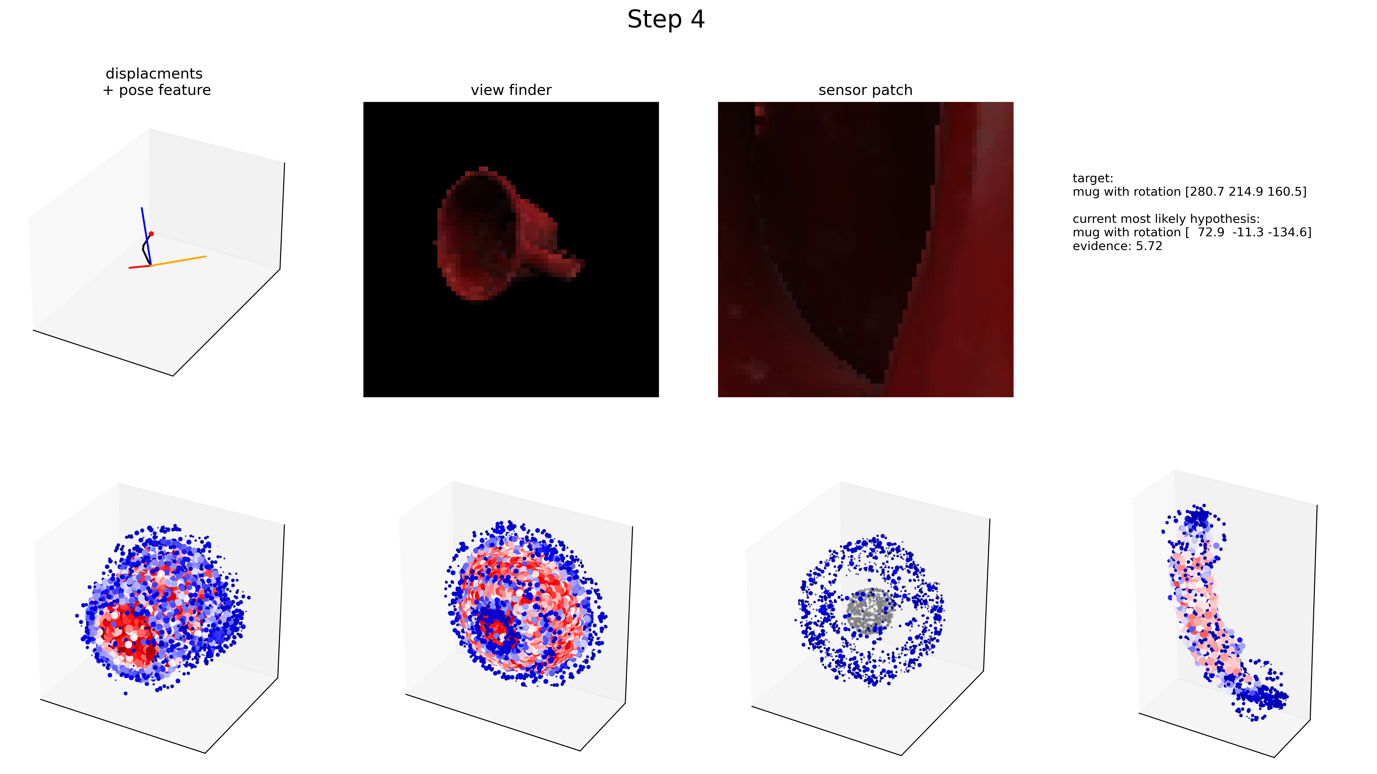
Data generated from an experiment using the EvidenceLM (currently the default setup) is best plotted using a loop, something similar as shown below. Note that you'll need to add code to define some of the placeholder variables.
from tbp.monty.frameworks.utils.plot_utils_dev import (
    plot_evidence_at_step,
    show_initial_hypotheses,
)

episode = 0
lm = "LM_0"
objects = ["mug","bowl","dice","banana"] # Up to 4 objects to visualize evidence for
current_evidence_update_threshold = -1
save_fig = True
save_path = exp_path + "/stepwise_examples/"

# [optional] Show initial hypotheses for each point on the object
show_initial_hypotheses(
    detailed_stats,
    episode,
    "mug",
    rotation=[120,-90],
    axis=2,
    save_fig=save_fig,
    save_path=save_path
)
# Plot the evidence for each hypothesis on each of the objects & show the observations used for updating
for step in range(eval_stats["monty_matching_steps"][episode]):
    plot_evidence_at_step(
        detailed_stats,
        lm_models,
        episode,
        step,
        objects,
        is_surface_sensor=True, # set this to False if not using the surface agent
        save_fig=save_fig,
        save_path=save_path
    )
The above code should create an image like the one shown below for each step in the experiment and save it in a folder called stepwise_examples inside the logs folder of this experiment.
Plotting Results (CSV)
Since the episode statistics are saved in a .csv table, you can also do all the standard plot visualizations of this data (such as bar plots of # episodes correct, # of steps per episode, ...). For example you could create the plot below using this code:
import matplotlib.pyplot as plt
import numpy as np
import seaborn as sns # For this you will have to install seaborn


rot_errs = np.array(eval_stats[eval_stats["primary_performance"]=="correct"]["rotation_error"])
rot_errs = rot_errs * 180 / np.pi

plt.figure(figsize=(12,5))
plt.subplot(1,2,1)
sns.histplot(rot_errs)
plt.xlabel("Rotation Error (degrees)")
plt.subplot(1,2,2)
sns.histplot(eval_stats, x="num_steps")
plt.xlabel("# of Steps")
plt.show()
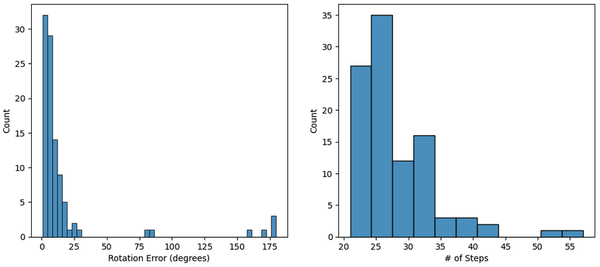
Obviously, there are tons of options for visualizing the logged data. The code and images above are just some examples to provide inspiration.
Analyzing Data From wandb_handlers
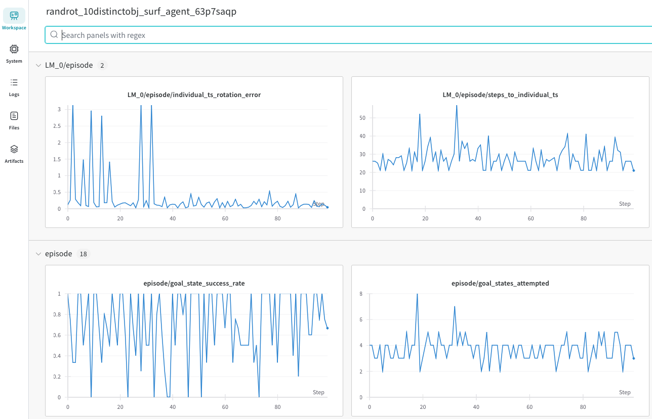
wandb_handlersWhen logging into Wandb, you can track your experiment results at https://wandb.ai/home . When you navigate to your project (by default called "Monty") you should see all your experiments in the Wandb dashboard. If you click on one of the runs, you should see something like this:
If you are using the BasicWandbTableStatsHandler, you will also see a table like this:
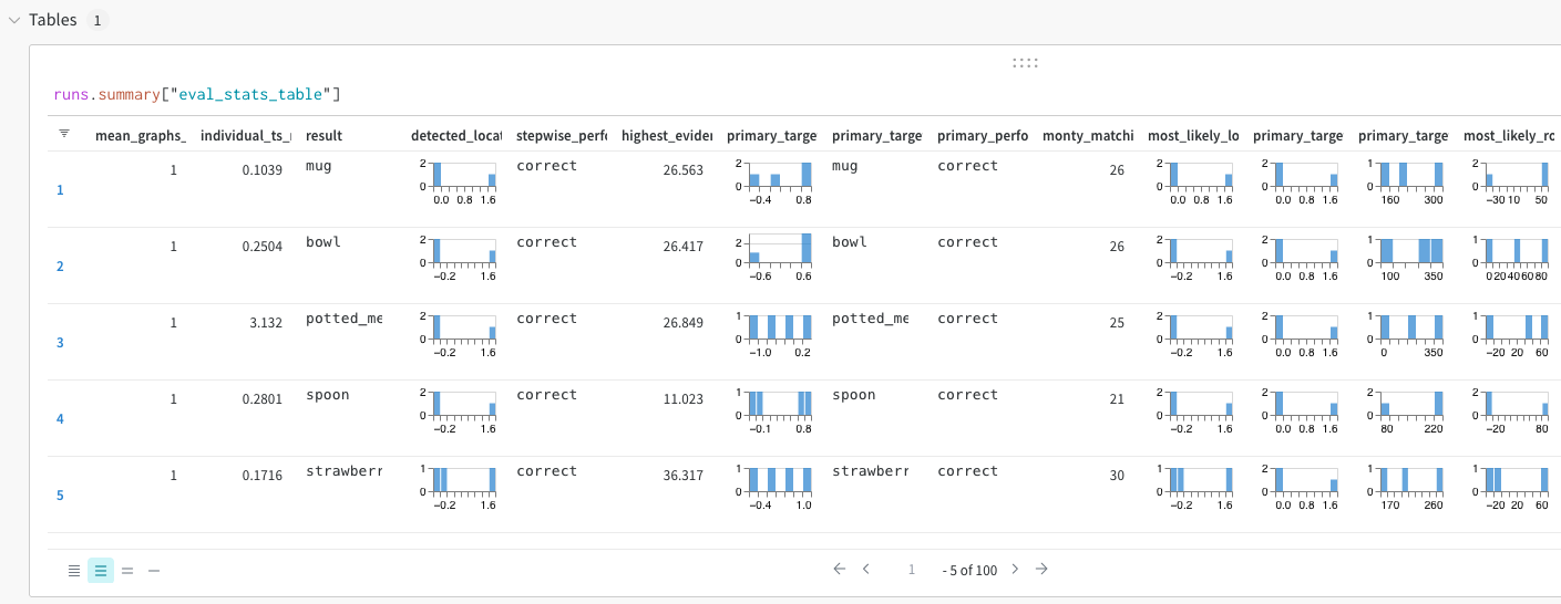
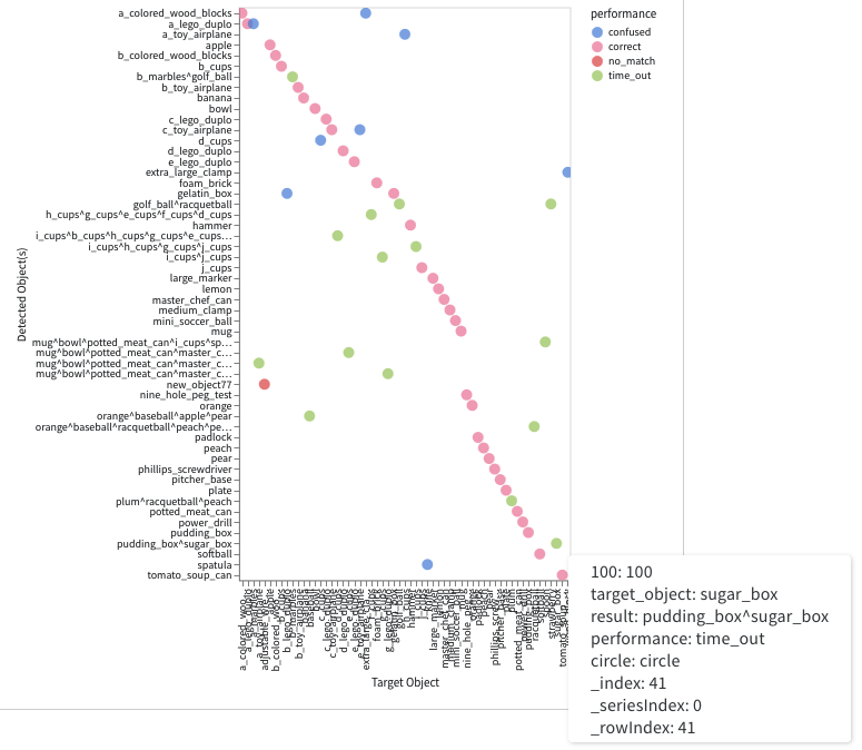
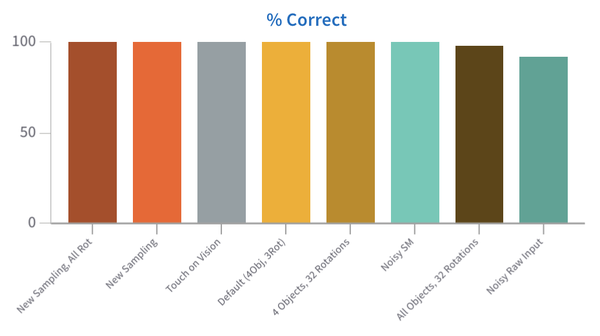
You can then create all kinds of plots from this data. A convenient way of doing this is using wandb reports but you can also create custom plots within the dashboard or download the data and plot it with any software of your choice.
Interactive Analysis with tbp.plot
tbp.plot
|
|
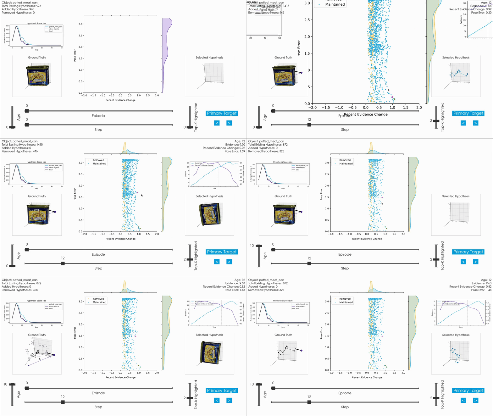
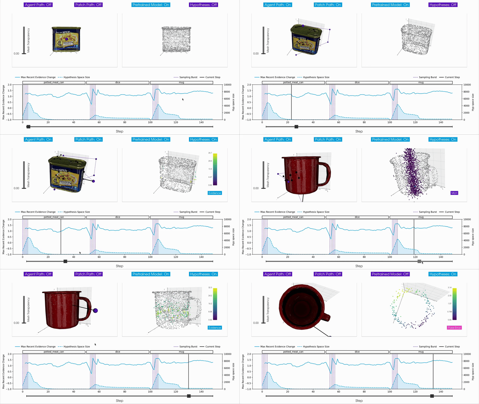
For interactive inspection, debugging and visualization of Monty experiment runs, we provide a separate companion repository called tbp.plot.
tbp.plot contains interactive visualization tools built on top of Vedo3D, which is a high-level wrapper for VTK. It allows you to visually interact with experiment logs by scrubbing through steps, visualizing the hypothesis space, inspecting meshes, and more. These tools are particularly useful when analyzing individual episodes to understand the evolution of hypotheses over time, or to debug unexpected behavior in an experiment run.
How to Use tbp.plot
tbp.plotA typical workflow is to first run a Monty experiment and then analyze the generated logs using tbp.plot. Most interactive visualizations rely on per-step data, so experiments are usually run with detailed logging enabled. In practice, this means running an experiment with the DetailedJSONHandler included in config.logging.monty_handlers, and keeping the number of episodes and objects small to keep the JSON log size manageable.
A quick and convenient way to achieve this is to override the configuration from the command-line interface, for example:
python run_parallel.py \
  experiment=randrot_noise_10distinctobj_dist_agent \
  episodes=\'5,9,12\' \
  +experiment/config/logging=detailed_evidence_lm
Tutorials and Examples
tbp.plot provides a set of tutorials that walk through how to build interactive visualizations from Monty experiment logs. These tutorials show how to load and parse the logs using DataParser and DataLocator helper classes and construct complex interactive widgets with pub/sub communication protocol.
You can find the tutorials and gallery of available tools in the tbp.plot repository.
Help Us Make This Page Better
All our docs are open-source. If something is wrong or unclear, submit a PR to fix it!
Updated 8 days ago
